import numpy as np
import matplotlib.pyplot as pltFilters
Low Pass RC Filter
# Low-pass filter transfer function

w = np.arange(1, 1000000, 1) * 2 * np.pi
R = 1e3
C = 0.1e-6
j = 1j
H = 1/(1 + j*w*R*C)

w_o = 1/(R*C)

# Plot the magnitude and phase of the transfer function
plt.figure()

plt.subplot(2, 1, 1)
plt.title('Low-pass filter transfer function')
plt.plot(w, np.abs(H))
plt.ylabel('|H|')
plt.xticks([])

# \omega_O is at the -3 dB point (1/sqrt(2) of the max)
plt.plot([w_o, w_o], [0, 1/np.sqrt(2)], color='yellow', linestyle='--')
plt.text(w_o, 1/np.sqrt(2), r'$\omega_0$', color='yellow')
plt.plot([0, w_o], [1/np.sqrt(2), 1/np.sqrt(2)], color='yellow', linestyle='--')
plt.xscale('log')

plt.subplot(2, 1, 2)
plt.plot(w, np.angle(H))
plt.ylabel(r'$\angle H$ (radians)')
plt.xlabel(r'$\omega$ (rad/s)')

# \omega_O is at the -45 degree point (-pi/4)
plt.plot([w_o, w_o], [-np.pi/2, -np.pi/4], color='yellow', linestyle='--')
plt.text(w_o, -np.pi/4, r'$\omega_0$', color='yellow')
plt.plot([0, w_o], [-np.pi/4, -np.pi/4], color='yellow', linestyle='--')
plt.xscale('log')

plt.savefig('../slides/images/rc_lpf_xfer_func.png', dpi=300, bbox_inches='tight')
plt.show()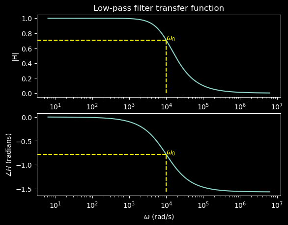
High Pass RC Filter
# High-pass filter transfer function

w = np.arange(1, 1000000, 1) * 2 * np.pi
R = 1e3
C = 0.1e-6
j=1j
H = (j*w*R*C)/(1 + j*w*R*C)

w_o = 1/(R*C)

# Plot the magnitude and phase of the transfer function
plt.figure()

plt.subplot(2, 1, 1)
plt.plot(w, np.abs(H))
plt.title('High-pass filter transfer function')
plt.ylabel('|H|')
plt.xticks([])

# \omega_O is at the -3 dB point (1/sqrt(2) of the max)
plt.plot([w_o, w_o], [0, 1/np.sqrt(2)], color='yellow', linestyle='--')
plt.text(w_o+2000, (1/np.sqrt(2)), r'$\omega_0$', color='yellow')
plt.plot([0, w_o], [1/np.sqrt(2), 1/np.sqrt(2)], color='yellow', linestyle='--')
plt.xscale('log')

plt.subplot(2, 1, 2)
plt.plot(w, np.angle(H))
plt.ylabel(r'$\angle H$ (radians)')
plt.xlabel(r'$\omega$ (rad/s)')

# \omega_O is at the -45 degree point (-pi/4)
plt.plot([w_o, w_o], [np.pi/2, np.pi/4], color='yellow', linestyle='--')
plt.text(w_o+500, (np.pi/4), r'$\omega_0$', color='yellow')
plt.plot([0, w_o], [np.pi/4, np.pi/4], color='yellow', linestyle='--')
plt.xscale('log')

plt.savefig('../slides/images/rc_hpf_xfer_func.png', dpi=300, bbox_inches='tight')
plt.show()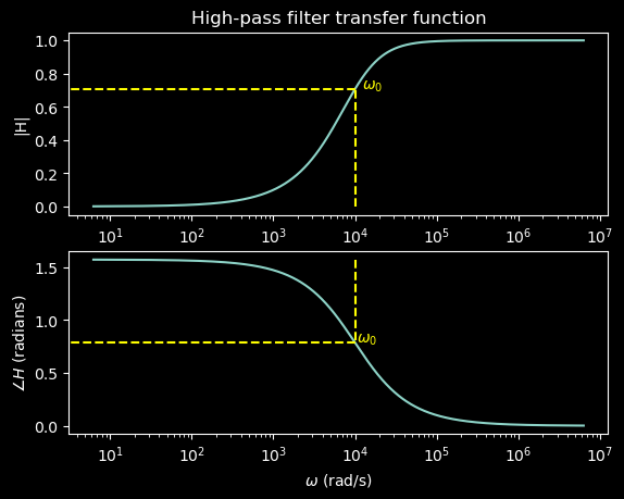
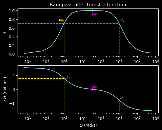
Bandpass Filter (Second-Order, RLC)
# Bandpass filter transfer function

w = np.arange(1, 10000000, 10) * 2 * np.pi
R = 10e3
C = 0.1e-6
L = 10e-3
j=1j
H = R/(R+(1/(j*w*C))+(j*w*L))

w_H = -R/(2*L) + np.sqrt((R/(2*L))**2 + 1/(L*C))
w_L = R/(2*L) + np.sqrt((R/(2*L))**2 + 1/(L*C))
w_o = np.sqrt(1/(L*C))

# Plot the magnitude and phase of the transfer function
plt.figure()

plt.subplot(2, 1, 1)
plt.plot(w, np.abs(H))
plt.title('Bandpass filter transfer function')
plt.ylabel('|H|')
plt.xticks([])

# \omega_H is at the -3 dB point (1/sqrt(2) of the max)
plt.plot([w_H, w_H], [0, 1/np.sqrt(2)], color='yellow', linestyle='--')
plt.text(w_H-500, (1/np.sqrt(2)+0.05), r'$\omega_H$', color='yellow')
plt.plot([0, w_H], [1/np.sqrt(2), 1/np.sqrt(2)], color='yellow', linestyle='--')
plt.plot([w_L, w_L], [0, 1/np.sqrt(2)], color='yellow', linestyle='--')
plt.text(w_L-500, (1/np.sqrt(2)+0.05), r'$\omega_L$', color='yellow')
plt.plot([0, w_L], [1/np.sqrt(2), 1/np.sqrt(2)], color='yellow', linestyle='--')
plt.scatter([w_o], [1], color='magenta', marker='x') # peak
plt.text(w_o, 0.9, r'$\omega_0$', color='magenta')

plt.xscale('log')

plt.subplot(2, 1, 2)
plt.plot(w, np.angle(H))
plt.ylabel(r'$\angle H$ (radians)')
plt.xlabel(r'$\omega$ (rad/s)')

# \omega_H is at the -45 degree point (-pi/4)
plt.plot([w_H, w_H], [-np.pi/2, np.pi/4], color='yellow', linestyle='--')
plt.text(w_H, (np.pi/4), r'$\omega_H$', color='yellow')
plt.plot([0, w_H], [np.pi/4, np.pi/4], color='yellow', linestyle='--')
plt.plot([w_L, w_L], [-np.pi/2, -np.pi/4], color='yellow', linestyle='--')
plt.text(w_L, (-np.pi/4-0.2)+0.3, r'$\omega_L$', color='yellow')
plt.plot([0, w_L], [-np.pi/4, -np.pi/4], color='yellow', linestyle='--')
plt.scatter([w_o], [0], color='magenta', marker='x') # peak
plt.text(w_o, 0.1, r'$\omega_0$', color='magenta')
plt.xscale('log')

plt.savefig('../slides/images/rc_bpf_xfer_func.png', dpi=300, bbox_inches='tight')
plt.show()