BME253L - Fall 2025
Duke University
October 6, 2025
The frequency response of a circuit is a measure of the variation of a load-related voltage/current signal as a function of the frequency content of the source signal.
Goal
Our goal is to evaluate the modulation of an input (voltage) signal by a circuit with frequency-dependent behavior leading to a frequency-dependent output (voltage) signal.
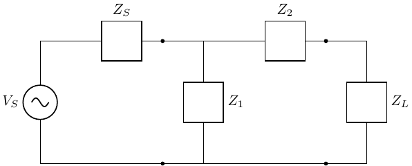
Generalized circuit block diagram with a source (input signal), a filter (circuit with frequency-dependent behavior), and a load (output signal).
A transfer function is a mathematical representation of the relationship between the input and output of a system as a function of frequency.
It describes how a filter modifies the amplitude and phase of the input signal to produce the output signal.
\[ \bar{H}(j\omega) = \frac{\bar{V}_{out}(j\omega)}{\bar{V}_{in}(j\omega)} \]
Complex quantity
Dimensionless
Function of frequency (\(\omega\))
\[ \begin{gather} V_{L} e^{j\phi_L} = |H|e^{j\angle H} V_{S} e^{j\phi_S} = |H| V_{S} e^{j(\phi_S + \angle H)} \\ V_{L} = |H| V_{S} \\ \phi_L = \angle H + \phi_S \end{gather} \]
Input/Source: all the stations broadcast span a wide range of frequencies in the FM band (88-108 MHz).
Desired Output/Load: a single station (e.g., 101.1 MHz).
Draw:
Input signal: multiple frequencies
Output signal: single frequency
Transfer function: band-pass filter centered at 101.1 MHz
Input/Source: music signal with a wide range of frequencies (bass, midrange, treble).
Desired Output/Load: enhanced bass and treble frequencies.
Draw:
Input signal: full spectrum
Output signal: enhanced bass and treble
Transfer functions: low-pass and high-pass filters
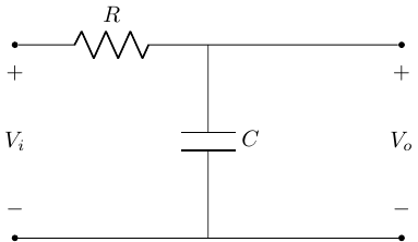
Let’s inspect the frequency response (transfer function) of this circuit…
\[ V_o = V_i \frac{\frac{1}{j\omega C}}{R + \frac{1}{j \omega C}} \\ \]
How did I get this expression?
\[ \frac{V_o}{V_i} = \frac{1}{1 + j\omega RC} \\ \]
Convert to polar form to get magnitude and phase:
\[ \begin{gather} |\bar{H}(j\omega)| = \frac{1}{\sqrt{1 + (\omega RC)^2}} \\ \angle \bar{H}(j\omega) = -\tan^{-1}(\omega RC) \\ \end{gather} \]
Let’s test some different frequencies to see what the transfer function tells us…
\[ \begin{gather} |\bar{H}(j0)| = 1 \\ \angle \bar{H}(j0) = 0^\circ \\ \end{gather} \]
That means that at DC, the output voltage is equal to the input voltage (no attenuation, no phase shift): \(V_o = V_i\). The capacitor is effectively an open circuit at DC.
\[ \begin{gather} |\bar{H}(j\infty)| = 0 \\ \angle \bar{H}(j\infty) = -90^\circ \\ \end{gather} \]
That means that at high frequencies, the output voltage is zero (completely attenuated) and the phase shift is -90 degrees: \(V_o = 0\). The capacitor is effectively a short circuit at high frequencies.
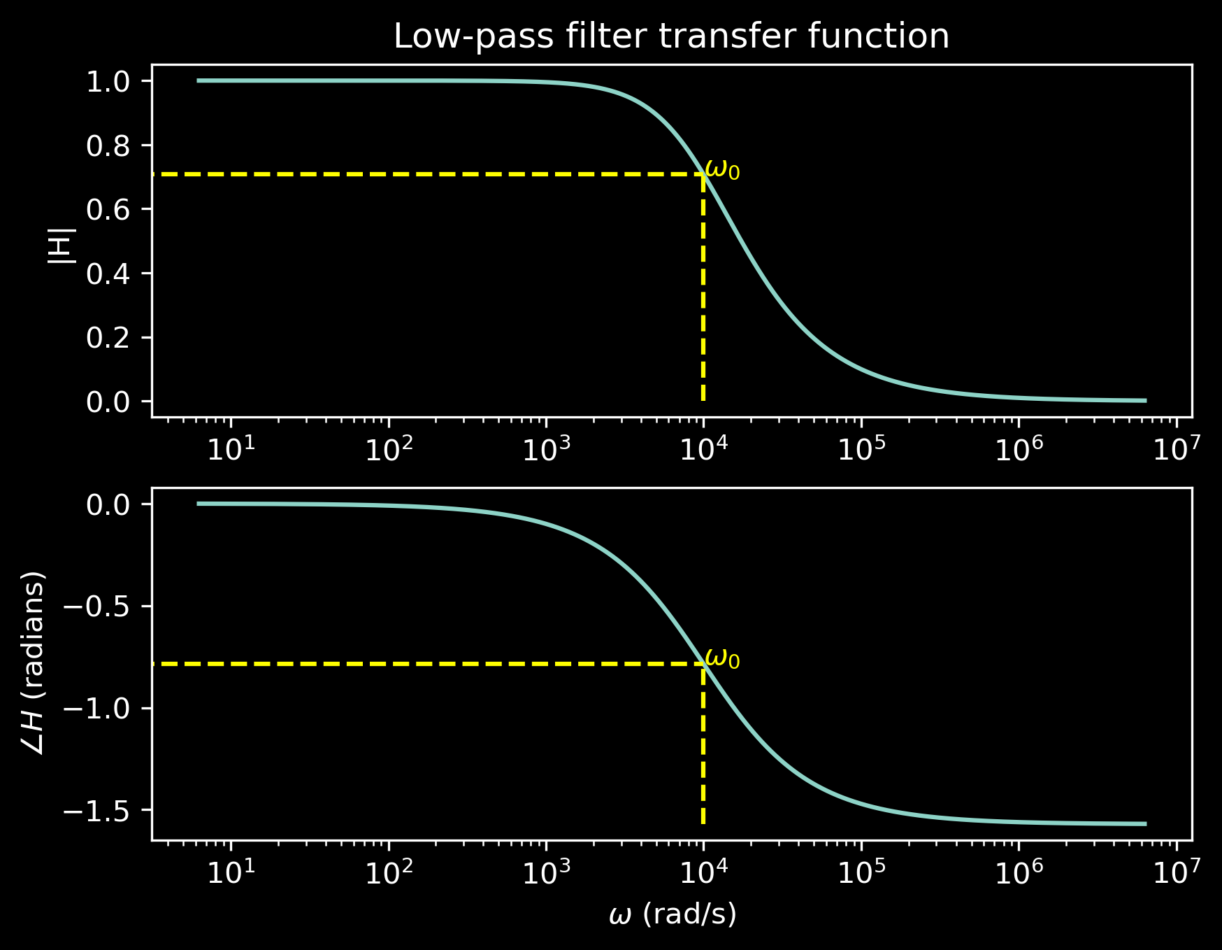
Note the logarithmic scale on the x-axis (frequency).
\(\omega_o\) is a characterisitic “cutoff” frequency that conveys information about the frequency response of the circuit.
\(V_o\) is at half power of \(V_i\) (\(|H| = 1/\sqrt{2}\)), which is attenuated by -3 dB (\(20 \log_{10}(1/\sqrt{2}) \approx -3\) dB).
The phase shift is -45 degrees (half of the total -90 degree shift).
Less-attenuated frequencies \(< \omega_o\) are in the passband.
More-attenuated frequencies \(> \omega_o\) are in the stopband.
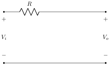
\[ \begin{gather} |\bar{H}(j\omega_o)| = \frac{1}{\sqrt{2}} = \frac{1}{\sqrt{1 + (\omega_o RC)^2}} \\ \omega_o = \frac{1}{RC} \end{gather} \]
Important
We can “tune” the frequency response of the filter by changing the values of \(R\) and \(C\)!
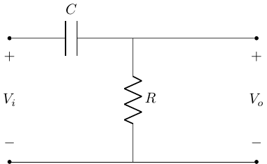
For \(\omega = 0\) (DC), the capacitor is an open circuit, so \(V_o = 0\).
For \(\omega = \infty\), the capacitor is a short circuit, so \(V_o = V_i\).
Higher frequency voltages are passed to the output, while lower frequency voltages are attenuated (taken up by the capacitor).
\[ \begin{gather} V_o(j\omega) = V_i(j\omega) \frac{R}{R + \frac{1}{j\omega C}} \\ H(j\omega) = \frac{j\omega RC}{1 + j\omega RC} \\ H(j\omega) = \frac{\omega RC}{\sqrt{1 + (\omega RC)^2}} \frac{\angle \frac{\pi}{2}}{\angle \tan^{-1}(\omega RC)} \\ |H(j\omega)| = \frac{\omega RC}{\sqrt{1 + (\omega RC)^2}} \\ \angle H(j\omega) = \frac{\pi}{2} - \tan^{-1}(\omega RC) \\ \end{gather} \]
Assume \(|H(j\omega)|_{max} = 1\) at \(\omega = \infty\).
\[ \begin{gather} |H(j\omega)| = \frac{|H(j\omega)|_{max}}{\sqrt{2}} \\ \frac{1}{\sqrt{2}} = \frac{\omega_o RC}{\sqrt{1 + (\omega_o RC)^2}} \\ \end{gather} \]
Important
\[ \omega_o = \frac{1}{RC} \\ \]
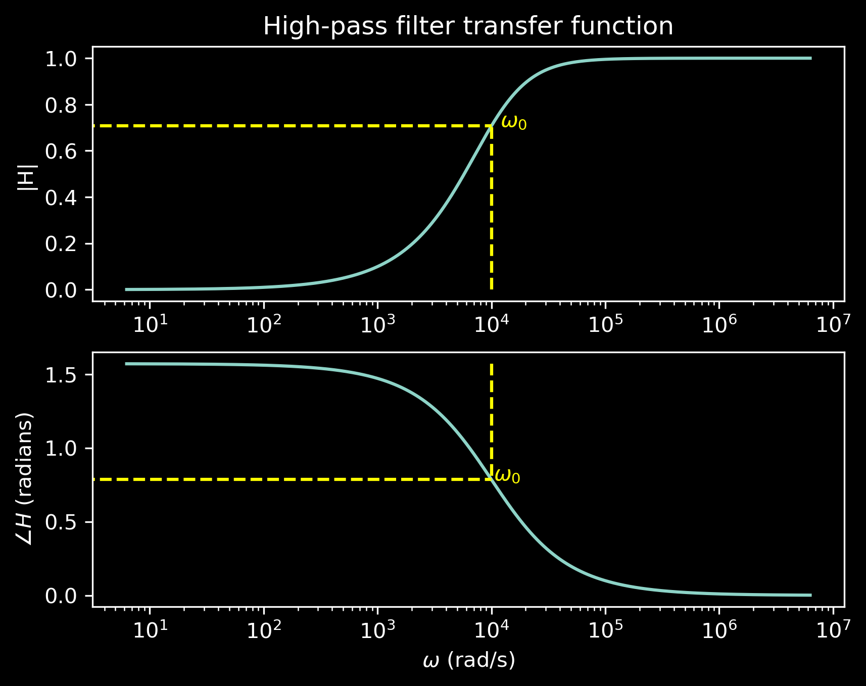
The passband is now frequencies \(>\omega_o\).
The stopband is now frequencies \(<\omega_o\).
In class demo…
Now that we are developing filters to modulate source signals to deliver to an attached load, we need to consider the impedances of the source, filter, and load.
The input impedance of the filter is the impedance “seen” by the source.
The output impedance of the filter is the impedance “seen” by the load.
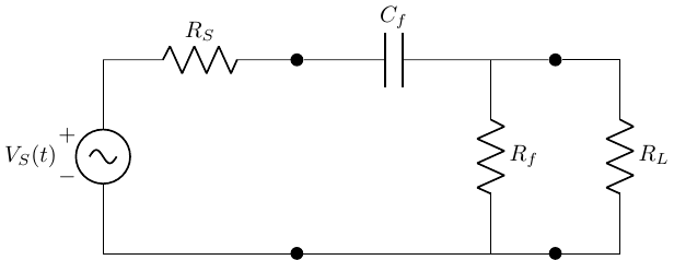
This can be considered a 3-stage circuit:
Source with internal impedance \(Z_S\).
Filter with input impedance \(Z_{in}\) and output impedance \(Z_{out}\).
Load with impedance \(Z_L\).
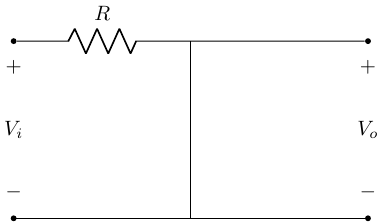
Remove the impedance of the load by replacing it with an open circuit.
Calculate the equivalent impedance of the filter that affects the current from the source.
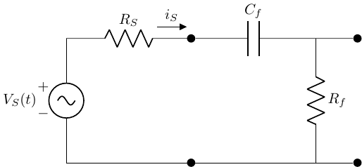
This is the input impedance of the filter, \(Z_{in}\).
\(Z_{in} = Z_f = Z_{C_f} + Z_{R_f}\) (as “seen” by the source)
\(Z_{in} = \frac{V_{in}}{I_{in}}\)
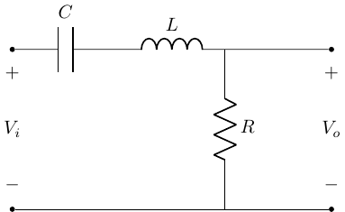
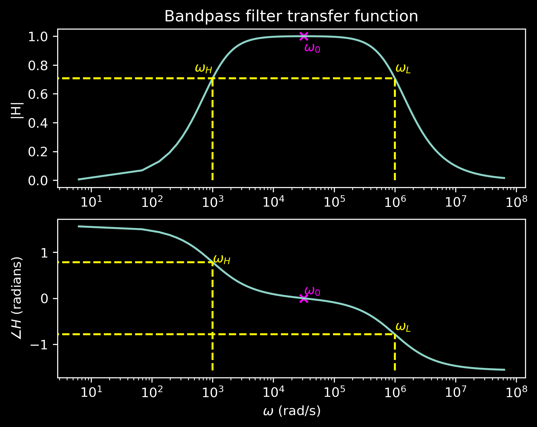
Important
If \(Z_{in} >> Z_L\), then the attached load will not affect the operation of the filter.
This means that we can cascade multiple filter stages without the load of one stage affecting the operation of the previous stage.
\[ Z_{out} = \frac{V_{oc}}{I_{sc}} \]
This is the Thevenin/Norton equivalent impedance “seen” by the load (which includes the source):
\[ \begin{gather} Z_{out} = {Z_{in}}_T \\ Z_{out} = Z_{R_f} || (Z_{R_S} + Z_{C_f}) \\ \end{gather} \]
Important
Note that \(Z_{in} \neq Z_{out}\)!
We can measure input and output impedance experimentally in the lab too.
Tip
This, again, just looks like a voltage divider!
This is a second-order filter (two energy storage elements: \(L\) and \(C\)), so it has two cutoff frequencies: \(\omega_H\) and \(\omega_L\).
\[ \begin{gather} H(j\omega) = \frac{V_o(j\omega)}{V_i(j\omega)} = \frac{R}{R + \frac{1}{j\omega C} + j\omega L} \\ H(j\omega) = \frac{j\omega RC}{1 + j\omega RC - \omega^2 LC} \\ \end{gather} \]
The bandwidth \(\Delta \omega\) is the difference between the upper and lower cutoff frequencies: \(\Delta \omega = \omega_H - \omega_L\).
The resonant frequency \(\omega_0\) is the frequency at which the inductive and capacitive reactances are equal in magnitude:
\[ \begin{gather} \omega_0 = \frac{1}{\sqrt{LC}} \\ \end{gather} \]
There are two points at which the power is half of the maximum power (or \(|H| = 1/\sqrt{2}\)):
\[ \omega_{L,H} = \pm \frac{R}{2L} + \sqrt{\left(\frac{R}{2L}\right)^2 + \frac{1}{LC}} \\ \]
Note
Note that you can view the bandpass filter as a cascade of a high-pass filter (formed by \(C\) and \(R\)) and a low-pass filter (formed by \(L\) and \(R\)), leading to a high- and low-frequency cutoff.
How “sharp” is the peak of the bandpass filter?
The quality factor \(Q\) is defined as:
\[ Q = \frac{\omega_0}{\Delta \omega} = \frac{\omega_0}{\omega_H - \omega_L} = \frac{1}{R} \sqrt{\frac{L}{C}} \\ \]
A higher \(Q\) indicates a sharper peak and a narrower bandwidth.
The damping factor \(\zeta\) is defined as:
\[ \zeta = \frac{1}{2Q} = \frac{R}{2} \sqrt{\frac{C}{L}} \\ \] It is a measure of how quickly oscillations in the system decay outside the passband.
Can we sketch transfer functions quickly without having to plot the exact function?
Yes! Bode plots provide a way to visualize the frequency response of a system using logarithmic scales for frequency and gain.
Decibel is a logarithmic unit used to express the ratio of two values, commonly power or intensity.
The formula to convert a power ratio to decibels is:
\[ L_{dB} = 10 \log_{10} \left( \frac{P}{P_0} \right) \]
where: - \(L_{dB}\) is the level in decibels, - \(P\) is the power being measured, - \(P_0\) is a reference power level.
For voltage gain, the formula is: \[ \left|\frac{V_{out}}{V_{in}}\right|_{dB} = 20 \log_{10} \left( \frac{V_{out}}{V_{in}} \right) \]
Why 20 and not 10?
Because power is proportional to the square of voltage (P ∝ V²), the factor of 20 accounts for this relationship when converting voltage ratios to decibels.
Allows a large dynamic range of signal levels to be represented in a “reasonable” linear range.
Example: hearing/sound intensity
Whisper: 0.00001 W/m² = -50 dB
Explosion: 100 W/m² = 100 dB
Exponential changes in power correspond to linear changes in dB, which is how our filters behave. We experience logarithmic changes in voltage as a function of decades of frequency change.
For a first-order low-pass filter, the Bode plot would show:
\[ \begin{align} \left|\frac{V_{out}}{V_{in}}\right|_{dB} & = -20 \log_{10} \left( \frac{1}{\sqrt{1 + \left( \frac{\omega}{\omega_c} \right)^2}} \right) \\ & = 20 \log_{10}(1) - 10 \log_{10}\left(1 + \left(\frac{\omega}{\omega_c}\right)^2\right) \\ & = -10 \log_{10}\left(1 + \left(\frac{\omega}{\omega_c}\right)^2\right) \\ \end{align} \]
For \(\frac{\omega}{\omega_c} << 1\), the gain is approximately \(-10 \log_{10}(1)\) = 0 dB (no attenuation).
For \(\frac{\omega}{\omega_c} >> 1\), the gain is approximately \(-10 \log_{10}((\frac{\omega}{\omega_c})^2)\) = -20 log₁₀(ω/ω_c) dB (attenuation increases with frequency).
A -20 dB/decade slope after the cutoff frequency.
A phase shift that approaches -\(\frac{\pi}{2}\) at high frequencies.
At the cutoff frequency (\(\omega = \omega_c\)):
The gain is -3 dB, and
The phase shift is -\(\frac{\pi}{4}\).
We simplify the transfer function into segments that are easy to plot, which intersect at the cutoff frequency.
The slope of the magnitude plot changes at the cutoff frequency.
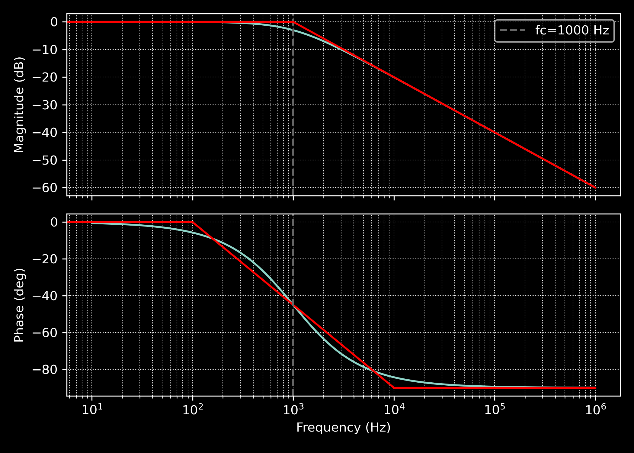
\(\frac{\omega}{\omega_c} << 1\): phase is approximately 0.
\(\frac{\omega}{\omega_c} >> 1\): phase is approximately -\(\frac{\pi}{2}\).
\(\omega = \omega_c\): phase is -\(\frac{\pi}{4}\).
Approximate the phase transition as linear over two decades centered at the cutoff frequency.
You tell me!
Solve for \(|H(j\omega)|\) and \(\angle H(j\omega)\).
Determine the cutoff frequency \(\omega_c\).
Evaluate \(|H(j\omega)|\) and \(\angle H(j\omega)\) at “extreme” frequencies (\(\omega << \omega_c\) and \(\omega >> \omega_c\)).
Sketch the magnitude and phase plots using straight lines that approximate the behavior of the transfer function, intersecting at \(\omega_c\).
For first-order filters, the slope of the magnitude plot changes by ±20 dB/decade at the cutoff frequency.
For first-order filters, the phase plot transitions from 0 to ±\(\frac{\pi}{2}\) degrees over two decades centered at the cutoff frequency.