Transient Analysis
BME253L - Fall 2025
Dr. Mark Palmeri, M.D., Ph.D.
Duke University
October 20, 2025
Overview
Unlike our filter analysis, which focused on steady-state sinusoidal inputs, transient analysis examines how circuits respond to time-varying signals, especially during switching events. This is crucial for understanding real-world circuit behavior, as many applications involve non-sinusoidal waveforms.
Learning Objectives
Understand how voltage and current change over time in response to switched DC sources in first-order and second-order, passive reactive circuits.
Evaluate transient response, analytically, using differential equations and initial conditions.
Numerically simulate transient response using SPICE.
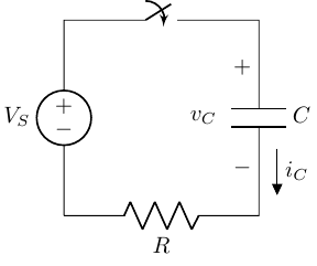
Switched RC Circuit
![]()
How can we model a closing switch mathematically?
Unit step function \(u(t) = \begin{cases} 0, & t < 0 \\ 1, & t \geq 0 \end{cases}\)o
Can scale and shift the unit step function to model a closing switch at \(t = t_0\):
\[
V_A u(t - t_0) = \begin{cases} 0, & t < t_0 \\ V_A, & t \geq t_0 \end{cases}
\]
In our example circuit:
Closing the switch at \(t = t_0\) can be modeled as \(V_S\,u(t - t_0)\).
Opening the switch at \(t = t_1\) can be modeled as \(V_S\,u(t - t_0) - V_S\,u(t - t_1)\).
Solving the Switched RC Circuit
We cannot use phasors here because the input is not steady-state sinusoidal.
Instead, we will use the IV relationships for resistors, capacitors and inductors to setup differential equations.
These differential equations will have general forms with known solutions that can be used to simplify the analsis, and we will leverage numerical solution using SPICE and scipy in your Jupyter notebooks.
Reminder: IV Relationships for Reactive Elements
\[
\begin{gather}
i_C(t) = C \frac{d v_C(t)}{d t} \\
v_C(t) = v_C(t_0) + \frac{1}{C} \int_{t_0}^{t} i_C(t) dt \\
\end{gather}
\]
\[
\begin{gather}
v_L(t) = L \frac{d i_L(t)}{d t} \\
i_L(t) = i_L(t_0) + \frac{1}{L} \int_{t_0}^{t} v_L(t) dt \\
\end{gather}
\]
Back to our Switched RC Circuit
![]()
KVL around the loop for \(t \geq t_0\):
\[
\begin{gather}
-V_S(t) + v_R(t) + v_C(t) = 0 \\
v_R(t) = i(t) R \\
i(t) = C \frac{d v_C(t)}{d t} \\
v_R(t) = R C \frac{d v_C(t)}{d t} \\
-v_S(t) + R C \frac{d v_C(t)}{d t} + v_C(t) = 0 \\
\Rightarrow R C \frac{d v_C(t)}{d t} + v_C(t) = V_S(t)
\end{gather}
\]
Lets solve for the natural response…
\[
\begin{gather}
\textrm{Remove the forced response:} v_i(t) = 0 \\
R C \frac{d v_n(t)}{d t} + v_n(t) = 0 \\
v_n(t) = A e^{st} \textrm{($s$ is a constant)}\\
R C A s e^{st} + A e^{st} = 0 \\
(R C s + 1) A e^{st} = 0 \\
\end{gather}
\]
\(A e^{st} \neq 0\) for all \(t\)
Characteristic Equation: \(R C s + 1 = 0 \Rightarrow s = -\frac{1}{R C} = -\frac{1}{\tau}\)
Natural Response: \(v_n(t) = A e^{-\frac{t}{\tau}} = A e^{-\frac{t - t_0}{\tau}}\)
\(A\) is determined by the initial condition \(v_n(t_0)\)
Now onto the forced response solution…
If \(v_i(t)\) is a DC source that is switched on at \(t = t_0\):
\[
v_i(t) = V_A u(t - t_0) = \begin{cases} 0, & t < t_0 \\ V_A, & t \geq t_0 \end{cases}
\]
\[
\begin{gather}
R C \frac{d v_f(t)}{d t} + v_f(t) = V_A \\
v_f(t) = V_A \textrm{(constant!)} \\
\frac{d v_f(t)}{d t} = 0 \\
R C (0) + V_A = V_A \\
V_A = V_A \\
\end{gather}
\]
Lets put our complete solution together…
\[
\begin{gather}
v_o(t) = v_n(t) + v_f(t) \\
v_o(t) = A e^{-\frac{t - t_0}{\tau}} + V_A \\
\end{gather}
\]
\[
\begin{gather}
v_C(t_0^-) = v_C(t_0^+) \Rightarrow v_C(t_0) = v_C(t_0^-) \\
A e^{-\frac{t_0 - t_0}{\tau}} + V_A = v_C(t_0^-) \\
A = v_C(t_0^-) - V_A \\
\end{gather}
\]
\[
v_C(t) = \left(v_C(t_0^-) - V_A\right) e^{-\frac{t - t_0}{\tau}} + V_A, \quad t \geq t_0
\]
Piecewise Linear (PWL) Sources
In-class demo. Take home points:
- Identify initial and steady-state conditions.
- Apply knowledge of the natural solution (exponential decay) between switching events.
- Apply forced response based on the new input after each switching event.
Second-Order Circuits
\[
a_2 \frac{d^2x(t)}{dt^2} + a_1 \frac{dx(t)}{dt} + a_0x(t) = b_0f(t)
\]
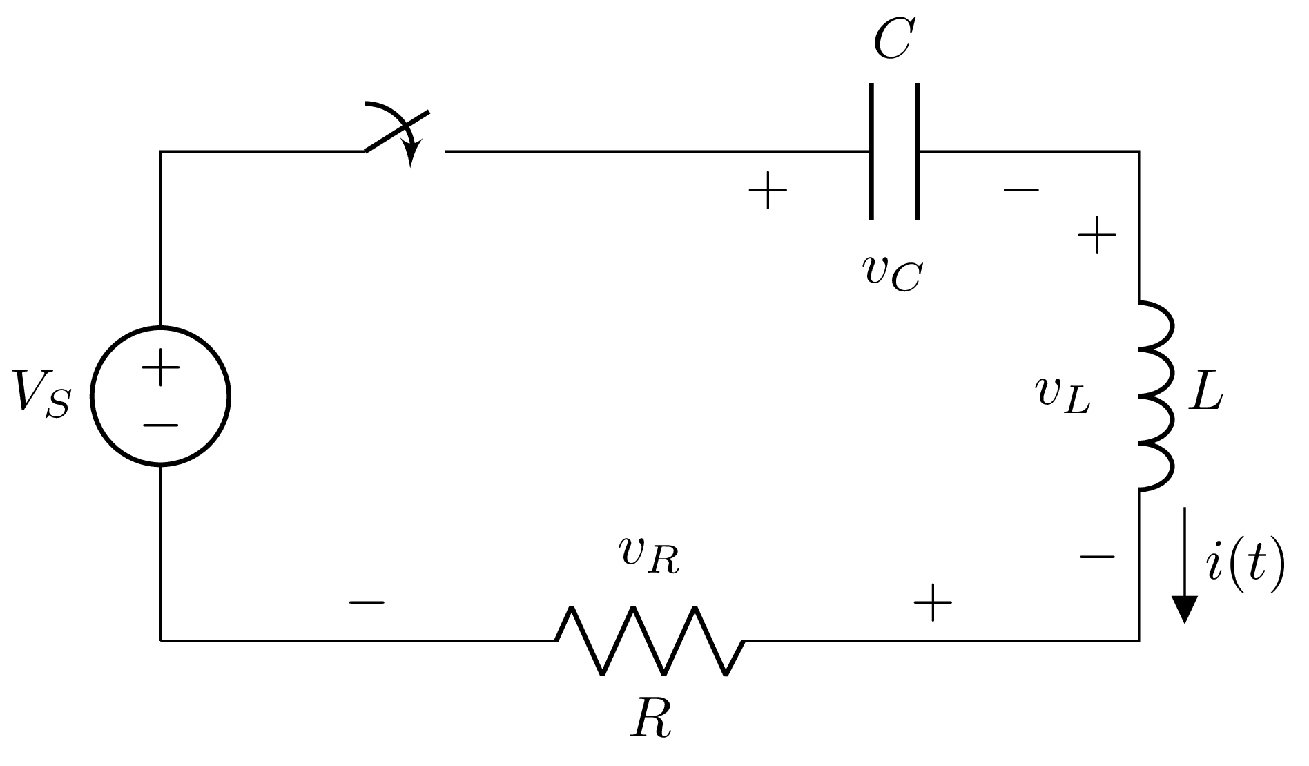
Switched RLC Circuit
![]()
Apply KVL around the loop for \(t \geq 0\):
\[
\begin{gather}
V_S - v_C(t) - v_L(t) - v_R(t) = 0 \\
v_R(t) = i(t) R \\
v_C(t) = \frac{1}{C} \int_{0}^{t} + v_C(0)\\
i(t) = C \frac{d v_C(t)}{d t} \\
v_L(t) = L \frac{d i(t)}{d t} \\
\end{gather}
\]
This yields:
\[
V_S(t) = i(t) R + L \frac{d i(t)}{d t} + \frac{1}{C} \int_{0}^{t} i(t) dt + v_C(0) \\
\]
But this is a mess to work with, so lets represent \(i(t)\) in terms of \(v_C(t)\):
\[
\begin{gather}
v_R = i(t) R = R C \frac{d v_C(t)}{d t} \\
v_L = L \frac{d i(t)}{d t} = L \frac{d}{d t} \left( C \frac{d v_C(t)}{d t} \right) = L C \frac{d^2 v_C(t)}{d t^2} \\
\end{gather}
\]
So we now have a second-order differential equation in terms of \(v_C(t)\):
\[
V_S(t) = L C \frac{d^2 v_C(t)}{d t^2} + R C \frac{d v_C(t)}{d t} + v_C(t)
\]
How do we solve this second-order differential equation?
\[
i_L(0) = i_C(0) = C \frac{d v_C(0)}{d t} \\
\]
Natural/Resonant Frequency
Damping Ratio
\(\zeta = \frac{R}{2} \sqrt{\frac{C}{L}}\) for a series RLC circuit.
Underdamped Solution (\(\zeta < 1\))
\[
\begin{gather}
v_C(t) = K e^{-\zeta \omega_n t} \cos(\omega_d t - \phi) \\
\omega_d = \omega_n \sqrt{1 - \zeta^2}
\end{gather}
\]
Critically Damped Solution (\(\zeta = 1\))
\[
\begin{gather}
v_C(t) = (A + B t) e^{-\omega_n t} \\
\end{gather}
\]
Overdamped Solution (\(\zeta > 1\))
\[
\begin{gather}
v_C(t) = A e^{s_1 t} + B e^{s_2 t} \\
s_{1,2} = -\zeta \omega_n \pm \omega_n \sqrt{\zeta^2 - 1} \\
\end{gather}
\]
Total Response
Sum of steady-state response and transient response (where the transient response is governed by one of the three cases above).
\[
v_C(t) = v_{steady-state}(t) + v_{transient}(t)
\]