Complex Impedance
BME253L - Fall 2025
October 1, 2025
What does this look like on the complex plane?
\(\bar{V}_R\) and \(\bar{I}_R\) are in phase.
Amplitude is governed by Ohm’s law: \(V_A = R I_A\).

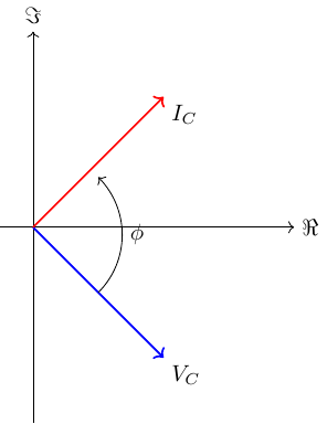
\(Z_c\) in the Time Domain
\[ \begin{gather} \bar{V}_c = \frac{\bar{I}_c}{j \omega C} = -j \frac{\bar{I}_c}{\omega C} = \frac{1}{\omega C} e^{-j \frac{\pi}{2}} (\bar{I}_c e^{j \phi}) \\ \bar{V}_c = \frac{I_c}{\omega C} e^{j(\phi - \frac{\pi}{2})} \\ \end{gather} \]
- Capacitor voltage lags current by \(\frac{\pi}{2}\) (90 deg).
Example: RC Circuit with a Switch
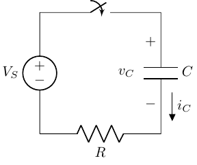
- The switch is closed at \(t=0\), connecting the voltage source to the series RC circuit.
\[ \begin{gather} v_C|_{t=0} = 0 \\ i_C = \frac{V_S}{R} \\ \end{gather} \]
The capacitor voltage cannot change instantaneously, so it starts at 0 V and behaves like a short circuit for an instant until it starts to accumulate charge.
As time evolves, the capacitor charges, and its voltage increases, reducing the current through the circuit.
\[ \begin{align} \bar{V}_L & = j \omega L \bar{I}_L = j \omega L (I_L e^{j\phi}) \\ & = \omega L I_L e^{\frac{\pi}{2}} e^{j\phi} \\ & = \omega L I_L e^{j(\phi + \frac{\pi}{2})} \\ \end{align} \]
The \(j\) indicates a phase shift of +90 degrees (voltage leads current).
The impedance is purely imaginary, indicating that the inductor does not dissipate energy but rather stores it in the magnetic field.

Example: RL Circuit with a Switch
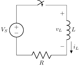
When the switch closes at \(t=0\):
\(v_L\) = \(V_S\) (initially behaves like an open circuit)
\(i_L\) = 0 A (initially no current through the inductor)
Example: RC Circuit AC Circuit Analysis
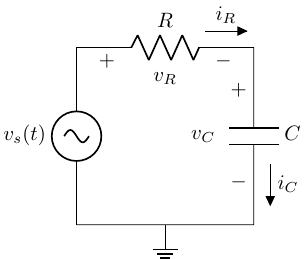
Solve for \(i_R(t)\) in the time domain (more painful).
\[ \begin{gather} i_R(t) = \frac{v_s(t) - v_C(t)}{R} \\ i_C(t) = C \frac{d v_C(t)}{dt} \end{gather} \]
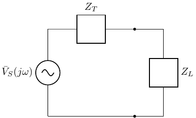
Complex Impedance Applied to Equiv. Circuits
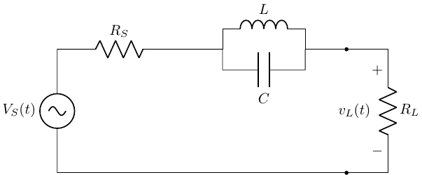
- Solve for Thevenin impedance (\(Z_{T}\)).
\[ \begin{align} Z_T & = Z_{R_S} + Z_L || Z_C \\ & = R_S + \left( \frac{1}{j \omega L} + \frac{1}{\frac{1}{j \omega C}} \right)^{-1} \\ & = R_S + \left( \frac{1}{j \omega L} + j \omega C \right)^{-1} \\ Z_T & = R_S + \frac{j \omega L}{1 - \omega^2 LC} \\ \end{align} \]
- Solve for Thevenin equivalent voltage (\(\bar{V}_{T}\)).
No current flows in the open-circuit load circuit, so: \[ v_{OC} = \bar{V}_S(j \omega) \]
The equivalent circuit is: